---
title: 'Übungszettel Principal Components Analyse und Faktoranalyse'
author: "Johannes Brachem (johannes.brachem@stud.uni-goettingen.de)"
subtitle: "M.Psy.205, Dozent: Peter Zezula"
output:
html_document:
theme: paper
toc: yes
toc_depth: 2
toc_float: yes
pdf_document: default
# latex_engine: xelatex
header-includes:
- \usepackage{comment}
params:
soln: TRUE
mainfont: Helvetica
linkcolor: blue
---
# Deutsch
## Links
[Übungszettel als PDF-Datei zum Drucken](https://pzezula.pages.gwdg.de/sheet_pca_fa.pdf)
`r if(!params$soln) {"\\begin{comment}"}`
**Übungszettel mit Lösungen**
[Lösungszettel als PDF-Datei zum Drucken](https://pzezula.pages.gwdg.de/sheet_pca_fa_solutions.pdf)
[Der gesamte Übugszettel als .Rmd-Datei](https://pzezula.pages.gwdg.de/sheet_pca_fa.Rmd) (Zum Downloaden: Rechtsklick > Speichern unter...)
`r if(!params$soln) {"\\end{comment}"}`
## Hinweise zur Bearbeitung
1. Bitte beantworten Sie die Fragen in einer .Rmd Datei. Sie können Sie über `Datei > Neue Datei > R Markdown...` eine neue R Markdown Datei erstellen. Den Text unter dem *Setup Chunk* (ab Zeile 11) können Sie löschen. [Unter diesem Link](https://pzezula.pages.gwdg.de/students_template.Rmd) können Sie auch unsere Vorlage-Datei herunterladen (Rechtsklick > Speichern unter...).
2. Informationen, die Sie für die Bearbeitung benötigen, finden Sie auf der [Website der Veranstaltung](https://www.psych.uni-goettingen.de/de/it/team/zezula/courses/multivariate)
3. Zögern Sie nicht, im Internet nach Lösungen zu suchen. Das effektive Suchen nach Lösungen für R-Probleme im Internet ist tatsächlich eine sehr nützliche Fähigkeit, auch Profis arbeiten auf diese Weise. Die beste Anlaufstelle dafür ist der [R-Bereich der Programmiererplattform Stackoverflow](https://stackoverflow.com/questions/tagged/r)
4. Auf der Website von R Studio finden Sie sehr [hilfreiche Übersichtszettel](https://www.rstudio.com/resources/cheatsheets/) zu vielen verschiedenen R-bezogenen Themen. Ein guter Anfang ist der [Base R Cheat Sheet](http://github.com/rstudio/cheatsheets/raw/master/base-r.pdf)
## Ressourcen
Da es sich um eine praktische Übung handelt, können wir Ihnen nicht alle neuen Befehle einzeln vorstellen. Stattdessen finden Sie hier Verweise auf sinnvolle Ressourcen, in denen Sie für die Bearbeitung unserer Aufgaben nachschlagen können.
Ressource | Beschreibung
-------------|--------------------------------
Field, Kapitel 17 | Buchkapitel, das Schritt für Schritt erklärt, worum es geht, und wie man Principal Components Analysen in R durchführt. **Große Empfehlung!**
## Tipp der Woche
Es gibt ein neues Paket namens `conflicted`, das Ihnen automatisch eine Fehlermeldung anzeigt, wenn Sie eine Funktion benutzen, die von zwei oder mehr Paketen verwendet wird. So werden Sie schnell auf potentiell nervtötende Flüchtigkeitsfehler aufmerksam gemacht. Alles, was Sie dafür tun müssen, ist das Paket zu installieren (`install.packages("conflicted")`) und zu Beginn Ihrer R-Skripte zu laden (`library(conflicted)`).
**Achtung** Wir haben Indizien dafür, dass ein laufendes `conflicted` die Stabilität von R unter Umständen stören kann. Wenn Sie den Verdacht haben, schalten Sie das Paket bitte vorsichtshalber aus. `detach(conflicted, unload=TRUE)`. Es gibt Alternativen, z. B. `conflicts(detail=TRUE)`, vgl.
[https://md.psych.bio.uni-goettingen.de/mv/unit/block_intro/block_intro_virt.html#command_masking](https://md.psych.bio.uni-goettingen.de/mv/unit/block_intro/block_intro_virt.html#command_masking)
**Beispiel**
```{r, eval = FALSE}
library(conflicted)
library(dplyr)
filter(mtcars, am & cyl == 8)
```

## 1) Daten einlesen, allgemeines zum Thema
1. Laden Sie die nötigen Pakete (dazu gehört heute auch `psych`) und setzen Sie ein sinnvolles Arbeitsverzeichnis.
2. Laden Sie den Datensatz `raq.dat` über den Link [https://pzezula.pages.gwdg.de/data/raq.dat](https://pzezula.pages.gwdg.de/data/raq.dat) herunter.
3. Lesen Sie den Datensatz unter dem Namen `raq_data` in R ein. Jede Zeile enthält die Antworten einer Versuchsperson.
4. Lesen Sie die Abschnitte "Überblick über die Items" und "Worum geht es?", um einen Überblick über die Thematik für diesen Übungszettel zu bekommen.
`r if(!params$soln) {"\\begin{comment}"}`
### Lösung
#### Unteraufgabe 1
```{r}
# Pakete laden
library(tidyverse)
library(psych)
```
```{r, eval = FALSE}
# Arbeitsverzeichnis setzen
# Ersetzen Sie hier den Dateipfad durch Ihren eigenen Dateipfad
setwd("~/ownCloud/_Arbeit/Hiwi Peter/gitlab_sheets")
```
#### Unteraufgabe 2
Bitte folgen Sie den Anweisungen in der Aufgabenstellung.
#### Unteraufgabe 3
```{r}
# raq_data <- read_delim("data/raq.dat", delim = "\t")
raq_data <- read_delim("http://md.psych.bio.uni-goettingen.de/mv/data/af/raq.dat", delim = "\t")
```
#### Unteraufgabe 4
Bitte folgen Sie den Anweisungen in der Aufgabenstellung.
`r if(!params$soln) {"\\end{comment}"}`
### Überblick über die Items
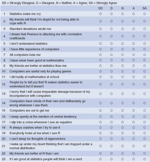
Der Datesatz enthält die Ergebnisse eines fiktiven Fragebogens (R Anxiety Questionnaire, RAQ) zur Angst vor Statistik (Field, S. 873). Hier sehen Sie die einzelnen Fragen.
### Worum geht es?
Dieser Übungszettel behandelt die explorative Faktorenanalyse (EFA) und die Hauptkomponentenanalyse (Principal Components Analysis, PCA).
Beide Verfahren dienen grob gesagt dazu, Variablen zu Gruppen zusammenzufassen. Dadurch kann man z.B. mit Multikollinearität (ein Problem von Regressionen, wenn mehrere Prädiktoren sehr hoch miteinander korrelieren) umgehen (PCA), oder nicht direkt beobachtbare (latente) Konstrukte erschließen (EFA). Mit der konfirmatorischen Faktoranalyse (Confirmatory Factor Analysis, CFA) können zusätzlich Theorien, die z.B. auf Grundlage von EFA aufgestellt wurden, überprüft werden.
Wir behandeln hier nur die ersten beiden Verfahren, also **Principal Components Analysis (PCA)** und **Exploratory Factor Analysis (EFA)**. Beide sind sich sehr ähnlich, tatsächlich kann die PCA als Sonderfall der EFA aufgefasst werden.
**Tabelle**: Übersicht über Faktoranalyse-Verfahren
Verfahren | Bedeutung | Anwendung
-------------|-------------------------------- |--------------------------------
Principal Components Analysis (PCA) | Variablen, die die gleiche Information beinhalten, werden zusammengefasst. | Bspw. zur Vermeidung von Multikollinearität in Regressionen.
Explorative Factor Analysis (EFA) | Variablen, die auf das selbe zugrundeliegende Merkmal, z.B. einer Person, zurückzuführen sind, werden zusammengefasst. | Bspw. Konstruktion von Fragebögen.
Confirmatory Factor Analysis (CFA) | Variablen, die auf das selbe zugrundeliegende Merkmal, z.B. einer Person, zurückzuführen sind, werden zusammengefasst. | Bspw. Test von Theorien über Faktoren
## 2) Erster Blick auf die Daten
Wie bei anderen Analysen auch müssen wir zunächst prüfen, ob die Daten überhaupt geeignet dafür sind, eine Faktoranalyse durchzuführen. Das heißt vor allem, dass wir überprüfen, ob es ausreichend Beziehungen zwischen den Daten gibt, die aber auch nicht zu stark sein dürfen. Wenn zwei Variablen praktisch identisch sind (Korrelation .90 oder höher), dann bereitet das der Analyse Probleme.
Wir inspizieren die Daten zunächst per Augemaß, führen dann einen Test durch und schauen uns zwei Indices an, die uns Informationen über die Angemessenheit einer Faktorenanalyse liefern.
Erklärungen dazu (nähere Information finden Sie in Field (2012)):
Kriterium | Bedeutung | Anwendung
-------------|-------------------------------- |--------------------------------
Korrelationsmatrix | Gibt es augenscheinlich angemessene Zusammenhänge zwischen den betrachteten Variablen? | Hinweise auf Probleme gibt es, wenn 1) Kaum Korrelation von .30 oder größer vorliegen, 2) (Viele) Korrelationen über .90 vorliegen, 3) Einzelne oder mehrere Variablen überhaupt nur sehr geringe Korrelationen mit allen anderen Variablen aufweisen.
Bartlett's Test | Handelt es sich bei der Korrelationsmatrix um eine Einheitsmatrix? | Wenn der Test signifikant wird, handelt es sich **nicht** um eine Einheitsmatrix. Das ist gut für die Faktorenanalyse. Ein nicht-signifikanter Test wäre ein Hinweis auf ein Problem.
Kaiser-Meyer-Olkin Maß (KMO) | Gibt es Muster in der Korrelationsmatrix, die durch Faktorenanalyse aufgedeckt werden können? | Kann Werte von 0-1 annehmen, je näher an 1, desto besser. Es gibt ein Gesamtmaß und Maße für jede einzelne Variable. Beide sollten betrachtet werden.
Determinante der Korrelationsmatrix | Sind die Beziehungen der Variablen in der Matrix stark (0) oder schwach (1)? | Die Determinante sollte klein, aber nicht kleiner als 0.00001 sein, damit eine Faktorenanalyse durchgeführt werden kann.
1. Nutzen Sie den Befehl `cor()`, um eine Korrelationsmatrix auf Grundlage des Datensatzen `raq_data` zu erstellen. *Tipp: Mit der Funktion `round()` können Sie die Ergebnisse abrunden, so dass sie leichter lesbar sind.*
2. Inspizieren Sie die Korrelationsmatrix, indem Sie einen Blick darauf werden. Gibt es einen Hinweis auf Probleme für die Faktorenanalyse?
3. Wenden Sie den Befehl `cortest.bartlett()` aus dem Paket `psych` auf den Datensatz oder auf die Korrelationsmatrix an (beides liefert identischer Ergebnisse, wenn der Datensatz ausschließlich dieselben Variablen enthält wie die Matrix). Gibt es einen Hinweis auf Probleme für die Faktorenanalyse? *Hinweis dazu:*
i) Wenn Sie die Funktion auf die Korrelationsmatrix anwenden, müssen Sie mit dem Argument `n = ` angeben, wie groß die Stichprobe ist.
4. Wenden Sie den Befehl `KMO()` aus dem Paket `psych` auf den Datensatz oder auf die Korrelationsmatrix an (beides liefert identischer Ergebnisse, wenn der Datensatz ausschließlich dieselben Variablen enthält wie die Matrix). Gibt es einen Hinweis auf Probleme für die Faktorenanalyse?
5. Wenden Sie den Befehl `det()` auf die **Korrelationsmatrix** an. Gibt es einen Hinweis auf Probleme für die Faktorenanalyse?
`r if(!params$soln) {"\\begin{comment}"}`
### Lösung
#### Unteraufgabe 1
```{r}
raq_matrix <- raq_data %>% cor() %>% round(2)
```
#### Unteraufgabe 2
a) Es gibt Korrelationen über .30
b) Es gibt keine Korrelationen über .90
c) Es gibt keine Variablen, die besorgniserregend wenig mit anderen korrelieren.
#### Unteraufgabe 3
```{r}
# Anwendung auf die Matrix
psych::cortest.bartlett(raq_matrix, n = 2571)
# Anwendung auf den Datensatz
psych::cortest.bartlett(raq_data)
```
Der Test ist signifikant: Es gibt Beziehungen zwischen den Daten.
#### Unteraufgabe 4
```{r}
# Anwendung der Funktion auf den Datensatz
kmo_raq <- psych::KMO(raq_data)
# Anzeigen der Ergebnisse
kmo_raq
# Anzeigen der Einzel-Werte in aufsteigender Reihenfolge
kmo_raq$MSAi %>% sort()
```
Der Gesamt-Wert liegt mit 0.93 im hervorragenden Bereich, und der geringste Einzelwert ist mit 0.77 immer noch im guten Bereich.
#### Unteraufgabe 5
```{r}
# Determinante der Korrelationsmatrix
det(raq_matrix)
```
Die Determinante ist klein, was auf starke Beziehungen zwischen den Variablen hindeutet. Gleichzeitig ist sie größer als der Cutoff von 0.00001, d.h. die Beziehungen zwischen den Variablen sind nicht *zu* stark.
Wir können hier also eine Faktoranalyse durchführen.
`r if(!params$soln) {"\\end{comment}"}`
## 3) Faktoren identifizieren
Bei explorativem Vorgehen wissen wir vor der Analyse nicht, wie viele Faktoren vorliegen. Wir nutzen zur Identifikation einen sogenannten *Scree-Plot* und die *Eigenvalues*, Werte aus einer ersten Analyse.
**Wir arbeiten hier zunächst nur mit der PCA. Das Vorgehen für die EFA ist beinahe identisch. Bei Unterschieden weisen wir darauf hin. In einer späteren Aufgabe thematisieren wir Unterschiede in den Ergebnissen.**
Der allgemeine Befehl für eine PCA in R stammt aus dem Paket `psych` und lautet:
`principal(r = , nfactors = , rotate = )`. Dabei steht `r` für die Korrelationsmatrix, bzw. die zugrundeliegenden Rohdaten, `nfactors` für die Anzahl von Faktoren, die wir identifiezieren möchten, und `rotate` für die Art der "Rotation". Die Rotation wird in einer späteren Aufgabe thematisiert.
Der Befehl für die explorative Faktorenanalyse ist genau gleich aufgebaut und lautet: `fa(r = , nfactors = , rotate = )`.
**Tabelle 3.1**: Wichtige Komponenten des Outputs einer PCA / EFA.
Komponente | Wo im Output? | Bedeutung
-------------|-----------------------------|--------------------------------
Faktorladungen (factor loadings) | Große Tabelle, oben im Output | Korrelation der jeweiligen Variable mit dem jeweiligen Faktor.
h2 | Am rechten Rand der Tabelle mit den Faktorladungen | *Communality*: Maß für den Anteil der Varianz der jeweiligen Variable, der durch die Faktoren des Modells erklärt werden kann.
u2 | Neben h2 | *Uniqueness*: Anteil einzigartiger Varianz der jeweiligen Variable. Berechnung als 1 - h2
Eigenvalues
(SS loadings) | Tabelle unter den Faktorladungen,
erste Zeile | Summe der quadrierten Faktorladungen pro Faktor. Werden dargestellt als Anteil erklärter Varianz. Bei 23 Variablen wie in unserem Fall entspricht ein eigenvalue von 7.29 (PC1) der Erklärung von 7.29 / 23 = 0.32, also 32% der Varianz in den Daten. Das ist auch in der zweiten Zeile der Tabelle abzulesen.
**Tabelle 3.2**: Kriterien zur Bestimmung der Anzahl sinnvoller Faktoren.
Kriterium | Welche Faktoren erhalten?
-------------|-------------------------------------------------------------
Kaiser | Faktoren mit Eigenvalue über 1
Wahrscheinlich ein gutes Kriterium, wenn weniger als 30 Variablen untersucht werden und die communalities *nach* der Faktor-Extraktion alle über 0.7 liegen. Wenn die Stichprobengröße über 250 liegt, sind auch communalities von 0.6 akzeptabel. Bei größeren Stichproben können wiederum noch kleinere communalities akzeptabel sein.
Jollife | Faktoren mit Eigenvalue über 0.7
Jollife war der Meinung, dass Kaisers Kriterium zu konservativ sei.
Scree Plot | Zeigt die Wichtigkeit aller Faktoren der ersten Analyse. Als Cut-Off wird der *point of inflexion* gewählt: Der Punkt, an dem sich die Steigung der Linie stark verändert, in der Regel von fast vertikal auf fast horizontal. Alle Faktoren links von diesem Punkt werden erhalten, die Faktoren rechts nichts.
1. Führen Sie eine PCA mit `raq_data` durch und speichern Sie diese unter dem Namen `pc1`. In der ersten Analyse möchten wir für `nfactors` die Gesamtzahl unserer untersuchten Variablen eingeben, in diesem Fall also 23. Für die Rotation wählen Sie zunächst bitte `rotate = "none"`.
i) **Achtung, Unterschied zur EFA**: In der EFA geben wir beim ersten Modell nicht die Gesamtzahl der Variablen ein, sondern einen geringeren Wert. In diesem Fall könnte man z.B. 18 eingeben.
2. Erstellen Sie einen Scree-Plot mit dem Befehl `plot(pc1$values, type = "b")`. Verstehen Sie den Code?
3. Betrachten Sie den Scree-Plot und die Eigenvalues im Output der PCA. Entscheiden Sie auf Grudlage von Tabelle 3.2, wie viele Faktoren Sie extrahieren möchten.
4. Führen Sie nun die PCA erneut durch, diesmal mit `nfactors = 4`, da wir vier Faktoren extrahieren möchten. Betrachten Sie die *communalities*. Ist die Extraktion von vier Faktoren nach Kaisers Kriterium gerechtfertigt?
a) Sie können zu diesem Zweck auch den Mittelwert der *communalities* betrachten.
5. Eine weitere, **sehr empfehlenswerte Methode** zur Bestimmung der Anzahl von Faktoren oder Hauptkomponenten ist die Parallel-Analyse. Dabei werden Zufallsdaten erzeugt und mit den realen Daten verglichen. Dieses Verfahren erlaubt eine weniger subjektive Entscheidung. Das Paket `psych` stellt mit dem Befehl `fa.parallel(, fa = <"method">)` eine unkomplizierte Methode zur Durchführung zur Verfügung. Setzen Sie für `` den Datensatz ein, und für `<"method">` die gewünschte Methode. In der PCA ist das `pc`, in den Faktorenanalyse `fa` (Sie können auch `both` eingeben). Führen Sie eine Parallel-Analyse für den vorliegenden Datensatz durch. Was ist Ihre Schlussfolgerung? (Näheres zur Interpretation finden Sie hier: [http://md.psych.bio.uni-goettingen.de/mv/unit/fa/fa.html#parallelanalyse](http://md.psych.bio.uni-goettingen.de/mv/unit/fa/fa.html#parallelanalyse))
6. Betrachten Sie die letzte Zeile des Outputs. Dort finden Sie ein weiteres Maß für die Passungs des Modells. Dieses Maß, wie so viele, geht von 0 bis 1. Je näher an der 1, desto besser ist die Passung des Modells auf die Daten. Werte über 0.95 werden generell als gute Passung angesehen. Eine genauere Erkläung zu diesem Wert finden Sie in Field (2012), S. 889 - 891.
`r if(!params$soln) {"\\begin{comment}"}`
### Lösung
#### Unteraufgabe 1
```{r}
# Analyse
pc1 <- psych::principal(raq_matrix, nfactors = ncol(raq_matrix), rotate = "none")
```
```{r}
# Output
pc1
```
#### Unteraufgabe 2
```{r}
# Ohne Pipe
plot(pc1$values, type = "b")
# Mit pipe
# pc1$values %>% plot(type = "b")
```
`pc1$values` greift auf das Objekt `values` im Output der PCA zu. `type = "b"` bedeutet, dass sowohl Punkte als auch Linien (**b**oth) geplotttet werden sollen.
#### Unteraufgabe 3
Der Scree-Plot wird relativ schnell flach, besonders allerdings nach dem 4. Faktor. Außerdem gibt es vier Faktoren mit Eigenvalues über 1, was nach Kaisers Kriterium passen würde. Nach Jollifes Kriterium würden wir 10 Faktoren extrahieren. Wir würden an dieser Stelle zunächst mit vier Faktoren weiterarbeiten, da Scree Plot und Kaisers Kriterium eher übereinstimmen. Es gibt hier kein völlig objektives Entscheidungskriterium, allerdings können wir in der Folge anhand der *communalities* überprüfen, ob die Entscheidung angemessen war.
Man kann anhand des Scree-Plots auch dafür argumentieren, dass nur zwei Faktoren extrahiert werden sollten. Probieren Sie das gerne auch selbst noch einmal aus!
#### Unteraufgabe 4
```{r}
# Analyse mit vier Faktoren
pc2 <- psych::principal(raq_data, nfactors = 4, rotate = "none")
# Output
pc2
# Mittlere communality
pc2$communality %>% mean()
```
Die mittlere communality ist mit .503 unter der Schwelle von .60, die für Kaisers Kriterium bei Stichproben ab 250 VP angegeben wird. Nach Field (2012) ist der Wert dennoch akzeptabel, da hier eine deutlich größere Stichprobe (n = 2571) vorliegt, für die diese Cut-Off-Werte vermtlich unterschritten werden dürfen. Darüber hinaus spricht auch der Scree-Plot tendenziell für die Extraktion von 4 Faktoren.
#### Unteraufgabe 5
```{r}
items_parallel <- psych::fa.parallel(raq_data, fa = "pc")
```
Auch die Parallelanalyse legt uns nahe, vier Faktoren (in diesem Fall *components*) zu extrahieren.
#### Unteraufgabe 6
Mit einem Wert von 0.96 weist das Modell eine gute Passung auf.
`r if(!params$soln) {"\\end{comment}"}`
## 5) Rotation und Scores
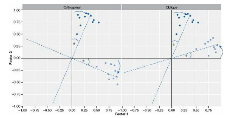
Faktorrotation ist ein wichtiger Schritt in der Faktorenanalyse, der es uns erlaubt, Faktoren deutlicher voneinander abzugrenzen. Das funktioniert durch eine Art "Drehung" (siehe Abbildung) des Koordinatensystem der Faktoren. Es gibt zwei Arten von Rotation:
Rotation | Bedeutung
-------------|-------------------------------------------------------------
Orthogonal | Faktoren werden rotiert, aber bleiben unabhängig voneinander (Korrelation = 0).
Oblique | Faktoren werden rotiert und dürfen miteinander korrelieren.
Genaueres können Sie in Field (2012), Kapitel 17.3.9 finden.
1. Führen Sie eine erneute PCA durch, und geben Sie bei diesem Mal `rotate = "varimax"` für die Rotation ein. Dadurch wird eine orthogonale Rotation durchgeführt. Speichern Sie die Analyse unter dem Namen `pc3`
a) Lassen Sie sich den Output mit dem Befehl `print.psych()` anzeigen. Wenn Sie dabei `cut = 0.3` und `sort = TRUE` als Argumente angeben, werden nur Faktorladungen ab 0.3 angezeigt, und die Variablen werden nach der Höhe ihrer Faktorladungen sortiert.
2. Wiederholen Sie den Schritt aus 1., geben Sie bei diesem Mal aber `rotate = "oblimin"` an und speichern Sie die Analyse unter dem Namen `pc4`.
a) Lassen Sie sich erneut den Output mit `print.psych()` anzeigen.
b) Vergleichen Sie den Output kurz mit dem Ouput von `pc3`
c) Der Output von pc4 enthält die Korrelationen der vier Faktoren. Können Sie diese im Output finden?
3. Sehen Sie sich nun die Fragen des RAQ an, die in `pc4` zu Faktoren zusammengefasst wurden.
a) Machen die Faktoren inhaltlich Sinn?
b) Wie würden Sie die Faktoren benennen?
c) Macht es inhaltlich Sinn, dass die Faktoren korrelieren dürfen? D.h. macht es Sinn, oblique Rotation zu verwenden?
d) Sind die Korrelationen zwischen den vier Faktoren inhaltlich sinnvoll?
4. *Factor Scores* enthalten die Werte einzelner Versuchspersonen für die extrahierten Faktoren. Extrahieren Sie die *Factor Scores* aus dem Output (`$scores`) und hängen Sie sie mit sinnvollen Variablennamen an den Rohdatensatz an. Geben Sie dem Objekt einen neuen Namen! **Achtung: Die Scores sind nur dann im Output-Objekt enthalten, wenn Sie den Rohdatensatz für die Analyse verwendet haben, nicht wenn Sie die Korrelationsmatrix verwendet haben.**
a) Haben Sie eine Idee, wie man in der Folge mit die *Factor Scores* verwenden könnte?
`r if(!params$soln) {"\\begin{comment}"}`
### Lösung
#### Unteraufgabe 1
```{r}
# Analyse durchführen
pc3 <- psych::principal(raq_data, nfactors = 4, rotate = "varimax")
# Output anzeigen
print.psych(pc3, cut = 0.3, sort = TRUE)
```
#### Unteraufgabe 2
```{r}
# Analyse durchführen
pc4 <- psych::principal(raq_data, nfactors = 4, rotate = "oblimin")
# Output anzeigen
print.psych(pc4, cut = 0.3, sort = TRUE)
```
#### Unteraufgabe 3
Die Faktoren scheinen inhaltlich Sinn zu ergeben. Field gibt Ihnen die Namen:
1. Fear of computers (TC1)
2. Fear of statistics (TC4)
3. Fear of mathematics (TC3)
4. Peer evaluation (TC2)
Da alle vier Faktoren Ängste beinhalten, ergibt es Sinn, dass sie miteinander korrelieren. Es ist daher auch inhaltlich sinnvoll, hier oblique Rotation einzusetzen.
Die relativ hohen Korrelationen zwischen TC1, TC4 und TC3 ergeben Sinn, da es sich um inhaltlich verwandte Konzepte handelt. Die geringeren Korrelationen mit TC2 erscheinen ebenfalls sinnvoll.
#### Unteraufgabe 4
```{r}
# Factor scores aus dem Modell extrahieren
scores <- pc4$scores
# Sinnvolle Spaltennamen vergeben
colnames(scores) <- c("fear_comp", "fear_stats", "fear_math", "fear_peer_eval")
# Scores und Rohdaten zusammenbinden
raq_data_scores <- cbind(raq_data, scores)
```
Die Faktorscores könnte man nun in der Folge z.B. als Prädiktoren in ein Regressionsmodell aufnehmen.
`r if(!params$soln) {"\\end{comment}"}`
## 6) Unterschied PCA - EFA
Der wichtigste theoretische Unterschied wurde oben bereits kurz erwähnt. Wir möchten durch diese Aufgabe nun noch einen praktischen Unterschied in den Fokus stellen.
1. Führen Sie eine EFA mit dem Befehl `fa()` aus dem Paket `psych()` durch. Verwenden Sie die gleichen Argumente, wie bei `pc2`, also ohne Rotation. Die Funktionen sind gleich aufgebaut. Speichern Sie das Ergebnis unter dem Namen `fa1`.
2. Führen Sie eine zweite EFA durch, und extrahieren Sie diesmal 10 Faktoren (nach Joliffes Kriterium). Speichern Sie das Ergebnis unter dem Namen `fa2`.
3. Führen Sie eine weitere PCA durch, und extrahieren Sie diesmal ebenfalls 10 Faktoren ohne Rotation. Speichern Sie das Ergebnis unter dem Namen `pc5`.
4. Verwenden Sie die Funktion `head()`, um sich die Faktor Scores für die ersten sechs VP anzeigen zu lassen.
a) Vergleichen Sie die Faktor Scores der ersten vier Faktoren in der Berechnung von `fa1` und `fa2`
b) Vergleichen Sie die Faktor Scores der ersten vier Faktoren in der Berechnung von `pc2` und `pc5`
c) Was fällt dabei auf?
`r if(!params$soln) {"\\begin{comment}"}`
### Lösung
#### Unteraufgabe 1
```{r}
fa1 <- psych::fa(raq_data, nfactors = 4, rotate = "none")
```
#### Unteraufgabe 2
```{r}
fa2 <- psych::fa(raq_data, nfactors = 10, rotate = "none")
```
#### Unteraufgabe 3
```{r}
pc5 <- psych::principal(raq_data, nfactors = 10, rotate = "none")
```
#### Unteraufgabe 4
```{r}
# a)
fa1$scores %>% head()
fa2$scores %>% head()
# b)
pc2$scores %>% head()
pc5$scores %>% head()
```
Die Faktor Scores der ersten vier Faktoren sind bei `fa1` und `fa2` unterschiedlich, während sie bei `pc2` und `pc5` gleich bleiben.
`r if(!params$soln) {"\\end{comment}"}`
## 7) Rendern
Lassen Sie die Datei mit `Strg` + `Shift` + `K` (Windows) oder `Cmd` + `Shift` + `K` (Mac) rendern. Sie sollten nun im "Viewer" unten rechts eine "schön aufpolierte" Version ihrer Datei sehen. Falls das klappt: Herzlichen Glückwunsch! Ihr Code kann vollständig ohne Fehlermeldung gerendert werden. Falls nicht: Nur mut, das wird schon noch! Gehen Sie auf Fehlersuche! Ansonsten schaffen wir es ja in der Übung vielleicht gemeinsam.
## Literatur
*Anmerkung*: Diese Übungszettel basieren zum Teil auf Aufgaben aus dem Lehrbuch *Dicovering Statistics Using R* (Field, Miles & Field, 2012). Sie wurden für den Zweck dieser Übung modifiziert, und der verwendete R-Code wurde aktualisiert.
Field, A., Miles, J., & Field, Z. (2012). *Discovering Statistics Using R*. London: SAGE Publications Ltd.
# English
## Links
[Exercise sheet as PDF](https://pzezula.pages.gwdg.de/sheet_pca_fa.pdf)
`r if(!params$soln) {"\\begin{comment}"}`
**Exercise sheet with solutions included**
[Exercise sheet with solutions included as PDF](https://pzezula.pages.gwdg.de/sheet_pca_fa_solutions.pdf)
[The source code of this sheet as .Rmdi](https://pzezula.pages.gwdg.de/sheet_pca_fa.Rmd)
(Right click and "save as" to download ...)
`r if(!params$soln) {"\\end{comment}"}`
## Some hints
1. Please try to solve this sheet in an .Rmd file. You can create one from scratch using `File > New file > R Markdown...`. You can delete the text beneath *Setup Chunk* (starting from line 11). Alternatively, you can download our template file unter [this link](https://pzezula.pages.gwdg.de/students_template.Rmd) (right click > save as...).
2. You'll find a lot of the important information on the [website of this course](https://www.psych.uni-goettingen.de/de/it/team/zezula/courses/multivariate)
3. Please don't hesitate to search the web for help with this sheet. In fact, being able to effectively search the web for problem solutions is a very useful skill, even R pros work this way all the time! The best starting point for this is the [R section on the programming site Stackoverflow](https://stackoverflow.com/questions/tagged/r)
4. On the R Studio website, you'll find highly helpful [cheat sheets](https://www.rstudio.com/resources/cheatsheets/) for many of R topics. The [base R cheat sheet](http://github.com/rstudio/cheatsheets/raw/master/base-r.pdf) might be a good starting point.
## Ressources
Since this is a hands-on seminar, we won't be able to present each and every new command to you explicitly. Instead, you'll find here references to helpful ressources that you can use for completing this sheets.
Ressource | Description
-------------|--------------------------------
Field, chapter 17 | Book chapter explaining step by step the why and how of principal component analysis in R.
**Highly recommended!**
## Hint of the week
There is a package named `conflicted` that automatically shows error messages when you use a function,
that exists in two or more packages. So your attention is drawn to errors of that type.
The only thing, you have to do, is to install this package (`install.packages("conflicted")`) and load it in your script (`require(conflicted)`).
**Example**
```{r, eval = FALSE}
library(conflicted)
library(dplyr)
filter(mtcars, am & cyl == 8)
```

## 1) Read data, some general remarks
1. Load the relevant packages, among these `psych` and set an adequate working directory.
2. Load the data set `raq.dat` from the link
[https://pzezula.pages.gwdg.de/data/raq.dat](https://pzezula.pages.gwdg.de/data/raq.dat)
and call the data object `raq_data`.
3. Each line has the answers of one subject.
4. Read the sections "Overview of the items" and "What is it about?" to get into the the topic.
`r if(!params$soln) {"\\begin{comment}"}`
### Solutions
#### Subtask 1
```{r}
# load packages
library(tidyverse)
library(psych)
```
```{r, eval = FALSE}
# set working directory
# put your directory here
setwd("P:/mv")
```
#### Subtask 2
See the instructions.
#### Subtask 3
```{r}
# this would be the syntax for locally stored data ...
# raq_data <- read_delim("data/raq.dat", delim = "\t")
# or
raq_data <- read_delim("https://pzezula.pages.gwdg.de/data/raq.dat", delim = "\t")
raq_data <- read_delim("http://md.psych.bio.uni-goettingen.de/mv/data/af/raq.dat", delim = "\t")
```
#### Subtask 4
See the instructions.
`r if(!params$soln) {"\\end{comment}"}`
### A look at the items
The data show answers to a fictive questionnaire, the "R Anxiety Questionnaire (RAQ)
with items for fear of statistics (Field, p. 873).
The items are:

### What is it about?
This exercise sheet is about explorative factor analysis (EFA) and principal component analysis (PCA).
Generally spoken, both are ways to aggregate variables to groups.
This helps us to treat mulicollinearity in multiple regression, when predictors correlate too high.
It is also useful to refer to latent constructs (f. e. traits) on base of indicator variables.
Moreover, we can use confirmatory factor analyses (CFA) to test theories that were set up on base of f. e. an EFA.
Here we only use the first two types, that is
**Principal Components Analysis (PCA)** and **Exploratory Factor Analysis (EFA)**.
Both are quite similar, indeed, we can look at PCA to be a special case of EFA.
**Table**: Overview on Types of Factor Analysis
Analysis | Meaning | Application
-------------|-------------------------------- |--------------------------------
Principal Components Analysis (PCA) | Variables, that share information, are aggregated | f. e. to deal with multicollinearity in regression analysis
Explorative Factor Analysis (EFA) | Variables, that base on the same hidden characteristic, are aggregated | f. e. construction of questionnaires
Confirmatory Factor Analysis (CFA) | Variables, that base on the same characteristic of f. e. a person, are aggregated. | f. e. tests of theories of factor structures.

## 2) A first look at the data
As with other analyses we have to check first, whether our data are suitable for factor analysis.
This means, whether we have sufficient but not too strong relations between the variables.
The analysis won't work, if two variables are practically identical (cor > .90).
Primarily we inspect the data manually, then we make a test and look at two indices,
that give us informations whether the data are suitable for factor analysis.
Some explanations (see Field (2012) for more information):
Criterium | Meaning | Application
-------------|-------------------------------- |--------------------------------
correlation matrix | Are there suitable correlations between our variables? | We have problems, if 1) we almost don't have correlations above 0.30. 2) We have (a lot of) correlations above .90. 3) Some of our variables have only very low correlations with all the others.
Bartlett's Test | Is our correlation matrix a singular matrix? | If the test is significant, we **don't** have singularity. This is, what factor analyses need. A non significant test would indicate problems.
Kaiser-Meyer Olkin measure (KMO) | Is there something systematic, that can be detected by applying a factor analysis. There is an overall index and an index for every variable. We should look at both.
Determinant of the correlation matrix | Are the relations in our correlation matrix strong (0) or weak (1)? | The determinant should be small, but not smaller than 0.00001, then a factor analysis is possible.
1. Use the command `cor()` to get a correlation matrix of `raq_data`.
*Tip: You can use `round()` to round numbers and make it more readable.*
2. Inspect the correlation matrix. Do you find anything that could cause problems running a factor analysis?
3. Run the command `cortest.bartlett()` of package `psych` on our data.
Run it on base of the data matrix or based on a correlation matrix.
Both ways should result in the same, if the variables contained are the same.
Do you see any problem applying factor analysis?
*a hint:* If your base is a correlation matrix, you have to specify argument `n = `
because your sample size is needed.
4. Apply `KMO()` of package `psych` to the data or to the correlation matrix.
Both ways should result in the same, if the variables contained are the same.
Do you see any problem applying factor analysis?
5. Apply `det()` to the **correlation matrix**.
Do you see any problem applying factor analysis?
`r if(!params$soln) {"\\begin{comment}"}`
### Solutions
#### Subtask 1
```{r}
raq_matrix <- raq_data %>% cor() %>% round(2)
```
#### Subtask 2
a) We find correlations above .30
b) We don't have correlations above .90
c) There are no variables, that call our attention, because they have only very low correlations with other variables.
#### Subtask 3
```{r}
# applying test to correlation matrix
psych::cortest.bartlett(raq_matrix, n = 2571)
# apply test to dataset
psych::cortest.bartlett(raq_data)
```
The test is significant. There are promising in the data.
#### Subtask 4
```{r}
# we apply the function to the dataset
kmo_raq <- psych::KMO(raq_data)
# ... and look at the results
kmo_raq
# we look at the values ordered increasingly
kmo_raq$MSAi %>% sort()
```
The overall index is 0.93 and the lowes single value is .77, which is still quite good.
Thus our indices show a high suitability for applying factor analysis to the data.
#### Subtask 5
```{r}
# the determinant of the correlation matrix
det(raq_matrix)
```
The determinant is small. That indicates strong relations between the variables.
But it's bigger than the recommended cutoff value of 0.00001.
This means, the relatins are not too strong in our data.
So we can conduct a factor analysis.
`r if(!params$soln) {"\\end{comment}"}`
## 3) Factor identification
When doing explorative analyses we don't know anything about the number of factors in our data.
We can use *scree plots* and *eigenvalues* of a first analysis to decide about that.
** We work here with PCA. With EFA the procedure is almost identical.
We will anounce differences.
An exercise below is dedicated to the differences in results.**
The general command for running a PCA in R is supplied by package `psych`:
`principal(r = , nfactors = , rotate = )`.
`r` refers to the correlation matrix or to the raw data matrix,
`nfactors` is the number of factors, that we want to extract.
`rotate` defines the type of rotation.
We talk about rotation later.
The structure of the command for running an EFA is the same:
`fa(r = , nfactors = , rotate = )`.
**Table 3.1**: Important components in the output of PCA/EFA.
Component | Where in the output? | Meaning
-------------|-----------------------------|--------------------------------
factor loadings | Big table up in the output | Correlations of the variables and the factors.
h2 | At the right of the table with factor loadings | *Cummunality*: Measure for the percentage of variance, that can be explained by the factors of the model.
u2 | right next to h2 | *Uniqueness*: Unique part of the variance of the variable in question. It's 1 - h2
Eigenvalues
(SS loadings) | table below the factor loadings,
first line | sum of the squared factor loadings per factor. It is shown as percentage of explained variance. In our case with 23 variables an eigenvalue of 7.29 (PC1) means 7.29 / 23 = 0.32 or 32% of the variance in the data. We can find that value in the second line of the table.
**Table 3.2**: Criteria to define an adequate number of factors to extract.
Criterion | Resulting number of factors to extract
-------------|-------------------------------------------------------------
Kaiser | Factors with eigenvalues above 1
presumably a good criterion if less than 30 variables are examined and the communalities *after* factor extraction are higher than 0.7. With sample sizes above 250 communalities of 0.6 are acceptable. With bigger samples we might accept even smaller communalities.
Jollife | Factors with eigenvalues above 0.7
in Jollife's opinion Kaiser's criterion was too conservative.
Scree Plot | Shows the importance of all factors of the first analysis. We look for a *point of inflexion*: A point, where the inclination of the resulting line changes rapidly. We can often detect a point, where the curve enters a sort of horizontal course after having started almost vertical. All Factors left of this point point of inflexion define the number of factors to extract.
1. Conduct a PCA on `raq_data` and store it under the name of `pc1`.
We want to have all possible factors included in the first analysis, this means a total of 23.
Please do not rotate, set `rotate = "none"`.
i) **Attention, difference to EFA**: In an EFA we do not extract as many factors
as our variables allow, we have to set a smaller number.
In this case, we could set it to 18 f. e..
3. Look at the scree-plot and at the eigenvalues in the output of PCA.
Decide on base of table 3.2 how many factors you want to extract.
4. Run the PCA again, but this time we want to extract four factors.
We set `nfactors = 4` to do that.
Look at the *communalities*.
Is the extraction of four factors correct if we refer to Kaiser Criterion?
a) You may have a look at the mean of the *communalities* to decide ...
5. A further and **very recommendable method** to decide about the number of facors in PCA
is the parallel-analysis.
Random data are generated repeatedly and compared to the real data.
This way the decision is not as subjective as the above mentioned possibilities.
Package `psych` offers an easy way to run it: `fa.parallel(, fa = <"method">)`.
Put in our data instead of `` and the method you want for `<"method">`.
For PCA you have to set `"pc"` and for FA `"fa"`. You may also put `"both"`.
Conduct a parallel-analysis on our dataset.
What is your conclusion?
(Find more on that under:
[http://md.psych.bio.uni-goettingen.de/mv/unit/fa/fa.html#parallelanalyse](http://md.psych.bio.uni-goettingen.de/mv/unit/fa/fa.html#parallelanalyse) )
6. Look at the last line of the output.
There you can find a further index for the fit of the model to the data.
This index varies between 0 and 1.
The closer to 1, the better the fit of model and data.
Values above 0.95 are considered to indicate a good fit.
Find a more in depth explanation for that in Field (2012, pp 889 - 891).
`r if(!params$soln) {"\\begin{comment}"}`
### Solutions
#### Subtask 1
```{r}
# Analysis
pc1 <- psych::principal(raq_matrix, nfactors = ncol(raq_matrix), rotate = "none")
```
```{r}
# Output
pc1
```
#### Subtask 2
```{r}
# without pipe
plot(pc1$values, type = "b")
# with pipe
# pc1$values %>% plot(type = "b")
```
`pc1$values` accesses object `values` in the output of our PCA. `type = "b"` means, that points and lines should be plotted (**b**oth).
#### Subtask 3
The scree plot gets to a more or less horizontal form quite fast, especially after the 4th factor.
Moreover we have four eigenvalues above 1, what would be congruent with the Kaiser Criterion.
Jollifes Criterion would suggest to extract 10 factors on the other hand.
We would keep on going with four factors at this point,
because of the congruence of the scree plot and Kaiser Criterion.
There is no objective decision but we can evaluate it by looking at the *communalities*.
Looking at the scree plot we could also have the impression of two factors beeing adequate.
Don't hesitate to try that also.
#### Subtask 4
```{r}
# Analysis with four factors
pc2 <- psych::principal(raq_data, nfactors = 4, rotate = "none")
# Output
pc2
# mean communality
pc2$communality %>% mean()
```
The mean communality of .503 is below .60,
which the recommended threshold of Kaiser Criterion for samples above 250 subjects.
Field (2012) considers this value acceptable, because our sample is way bigger than that (n=2571).
So our cut off values will presumably passed in this case.
We can also interprete our scree plot as an hint to extract 4 factors.
#### Subtask 5
```{r}
items_parallel <- psych::fa.parallel(raq_data, fa = "pc")
```
For PCA also our parallel analysis recommends the extraction of four *components*.
#### Subtask 6
Our model has an fit index of 0.96, which is considered a good fit.
`r if(!params$soln) {"\\end{comment}"}`
## 5) Rotation and scores
Factor rotation is an important step in factor analysis,
that allows us to separate factors more clearly from each other.
This works by a sort of multidimensional rotation of the coordinate system of the factors.
There are two types of rotation:
Rotation | Meaning
-------------|-------------------------------------------------------------
Orthogonal | Factors are rotated, but stay independent (orthogonal) from each other. Their intercorrelation is 0.
Oblique | Faktors are rotated and correlations between the rotated factors are allowed.
Find more about this in Field (2012) chapter 17.3.9

1. Make a new PCA and use `rotate = "varimax"` to get factor rotation.
This will make an orthogonal rotation.
Store the result and name it `pc3`.
a) Generate the output via `print.psych()`.
If you add the arguments `cut = 0.3` and `sort = TRUE`, only factor loadings above 0.3 are shown and
the factors are sorted by factor loading.
2. Repeat the steps of 1. but add `rotate = "oblimin"` this time, store the result and name it `pc4`.
a) Again, get the output using `print.psych()`.
b) compare the new output with `pc3`.
c) Find the correlations of the four factors in the output of `pc4`.
3. Take a look at the questions of RAQ and how they were clustered in `pc4` into factors.
a) Does the combination of items to factors make sense to you?
Can you find a common content in the combined questions?
b) What would you call the factors? Name them.
c) Makes it sense to let the factors correlate?
In other words, does oblique rotation make sense?
d) If you think of the content they have: Do the correlations found between the four factors make sense?
4. *Factor Scores* indicate the level of our obervations in our factors.
Extract the *Factor Scores* from our output (`$scores`) and add them to our data object giving them adequate names.
Give a meaningful name to our newly structured data object.
**Take care: We can only find our factor scores in our ouput object,
when we used raw data to do the factor analysis.
If we started using a correlation matrix, they are not computed.
a) Do you have any idea what we could use factor scores for?
`r if(!params$soln) {"\\begin{comment}"}`
### Solutions
#### Subtask 1
```{r}
# do the analysis
pc3 <- psych::principal(raq_data, nfactors = 4, rotate = "varimax")
# show the output
print.psych(pc3, cut = 0.3, sort = TRUE)
```
#### Subtask 2
```{r}
# do the analysis
pc4 <- psych::principal(raq_data, nfactors = 4, rotate = "oblimin")
# show the output
print.psych(pc4, cut = 0.3, sort = TRUE)
```
#### Subtask 3
The factors found seem to be meaningful. Field names them:
1. Fear of computers (TC1)
2. Fear of statistics (TC4)
3. Fear of mathematics (TC3)
4. Peer evaluation (TC2)
As all of the factors are variations of some type of fear, accepting correlations between them make sense.
So it's adequate to run oblique rotation.
The relatively high intercorrelations of TC1, TC3, and TC4 also make sense,
because they are conceptually close to each other.
This holds also for the low correlations they have with TC2.
#### Subtask 4
```{r}
# extract factor scores from the result object
scores <- pc4$scores
# we set meaningful columng names
colnames(scores) <- c("fear_comp", "fear_stats", "fear_math", "fear_peer_eval")
# we add the factor scores to our data table
raq_data_scores <- cbind(raq_data, scores)
```
We could use the factor scores f. e. in a regression, where we use them as predictors (explanatory variables).
`r if(!params$soln) {"\\end{comment}"}`
## 6) Differences between PCA and EFA
The most significant difference was mentioned above already.
Here we want to focus on a more practical aspect.
1. Conduct an EFA using the command `fa()` of package `psych()`.
Use the same arguments you had in `pc2`, also without rotation.
The commands have the same structure.
Store the result and name it `fa1`.
2. Run a second EFA and ectract 10 factors this time.
This would be the recommendation of the Joliffes Criterion.
Store the result and name it `fa2`.
3. Run another PCA and extract 10 factors without rotationg them.
Store the result and name it `pc5`.
4. Use the function `head()` to inspect the factor scores of the first 6 subjects (observations).
a) Compare the factor scores of the first four factors in the results of `fa1` and `fa2`.
b) Compare the factor scores of the first four factors in the results of `pc2` and `pc5`.
c) Is there anything special, you notice?
`r if(!params$soln) {"\\begin{comment}"}`
### Solutions
#### Subtask 1
```{r}
fa1 <- psych::fa(raq_data, nfactors = 4, rotate = "none")
```
#### Subtask 2
```{r}
fa2 <- psych::fa(raq_data, nfactors = 10, rotate = "none")
```
#### Subtask 3
```{r}
pc5 <- psych::principal(raq_data, nfactors = 10, rotate = "none")
```
#### Subtask 4
```{r}
# a)
fa1$scores %>% head()
fa2$scores %>% head()
# b)
pc2$scores %>% head()
pc5$scores %>% head()
```
The factor scores of the first four factors differ between `fa1` and `fa2`,
wheras they keep the same in `pc2` and `pc5`.
`r if(!params$soln) {"\\end{comment}"}`
## 7) Rendering
Render or knit your Rmd file using the shortcut `strg` + `shift` + `k` (Windows) or `cmd` + `shift` + `k`.
If that works: Well done!
If not, look at the error message, in special the lines in the syntax, where the error occured.
Correct the error and start over again.
We can help you in our exercise hour.
## Literature
*Annotation*: This exercise sheet is based in part on the exercises from the textbook
*Dicovering Statistics Using R* (Field, Miles & Field, 2012).
We modified it for the purpose of this exercise and actualized the R-Code.
Field, A., Miles, J., & Field, Z. (2012). *Discovering Statistics Using R*. London: SAGE Publications Ltd.